HENI Auction Index Methodology

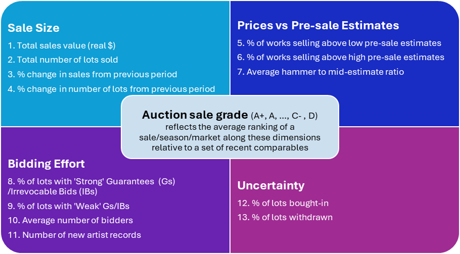
Auction Sale Characteristics

Each sale is categorised by a vector of sale characteristics related to four dimensions:

Notes:

1. Guarantees and IBs

A higher number of lots with Guarantees (Gs) and Irrevocable Bids (IBs) can be viewed:

• Positively: reflecting strong demand, confidence among buyers

• Negatively: uncertainty (auction houses often seek third-party guarantees when there is uncertainty over whether a lot will sell at auction), lack of confidence among sellers (guarantees are used to encourage consignments)

To distinguish both cases we define two separate metrics:

• ‘Strong’ Gs/IBs = lots with an IB or G selling above the high estimate

• ‘Weak’ Gs/IBs = lots with an IB/G selling at or below the low estimate

2. Real total sales value

Since we compare total sales values over long periods of time (up to two decades in some cases), it is important to adjust total sales for inflation (we use US CPI).

3. Collection sales

We select all collection sales that totalled at least $10mn in real terms.

When applying the algorithm to collection sales, we drop metrics 3 and 4 because percentage changes from previous make less sense with collection sales that happen throughout the year and many smaller sales happening in-between larger ones.

Sales Ranking Algorithm

To rank sales, we run the following straightforward algorithm on the set of most recent comparable sales†:

Step 1: rank all sales for each characteristic separately

• The rank is produced such that the higher the characteristic the higher the rank, i.e. characteristics 9, 12, and 13 are inverted as higher values indicate worse outcomes
• Characteristics where data is missing for more than 50% of the sample are dropped

Step 2: transform ranks into percentiles

Since some sales lack complete characteristic data, percentiles ensure our metric remains consistent regardless of sample size

Step 3: take the average of percentile rankings (= Sale Score)

We call this average the overall ‘Sale Score’. This step ensures that we could have different numbers of ranking characteristics over time (e.g. the number of bidders is a metric that is not available for all sales)

Step 4: transform the Sale Score into a percentile and translate into a Sale Grade

This step is akin to ‘grading on a curve’ and ensures that if Sale Scores are clustered around a specific value, we are still able to disentangle good and bad sales. We transform the percentile of the Sale Score into a Sale Grade using the following correspondence:

† For regular sales that happen 1 – 4 times per year we use a sample of 20 most recent sales. A larger number would make us go too far back into history and sometimes is not available at all. For collection sales where we have a larger sample, we go up to 100.

Using a rolling window of most recent sales to classify each new sale ensures that:

1. the resulting classification is point-in-time (i.e. a given sale’s classification does not use any look-ahead information, and a sale is not re-classified later on).
2. our algorithm takes into account the evolving nature of the art market, i.e. what used to be a B sale could today have become an A or C sale.

As robustness checks, we tried other rolling windows to confirm that grade changes are minimal, and qualitative conclusions remain the same. Note also that till we reach the required sample size, the algorithm uses an expanding set of sales, with a minimum of 5 sales required to produce a classification.